Excel 2016 charts: How to use the new Pareto, Histogram, and Waterfall formats

Excel 2016’s many new features include six new chart types. We’ll go over Histogram, Pareto, and Waterfall and talk about how they could be used with your data. We covered Treemap, Sunburst, and Box & Whisker earlier.

Histogram shows ranges of values

The Histogram chart in Excel 2016 looks like a regular column chart, but each column represents a ‘range’ of values (called a bin) instead of a single value. Histogram charts are for exploring and analyzing the frequencies within a distribution, statistics, density estimation, etc. Histograms also show results of continuous data such as height, weight, distance, etc.

1. Open your spreadsheet and select the database. Click Insert > Insert Statistical Chart > Histogram. The chart drops in and opens the Chart Tools/Design Ribbon menus. Scroll across the Design options and select one that fits your project.

2. Click the + sign to edit the chart elements, then click the paintbrush to change the chart’s style, design, or colors. The style changes are subtle, such as location of the legend, or font attributes. Browse through the options and choose your favorite.

3. Right-click any of the rectangles on the chart and select Format Data Series. In the Format Data Series pane, click Series Options (the chart icon).

4. Click the down arrow beside Series Options and browse through the drop-down menu to ascertain how each of these options perform. Select Horizontal Category Axis from the list.

5. Under Axis Options, select Number of Bins and change it to 10. For the Overflow bin, enter 850.0; for Underflow bin, enter 100.0. For Tick Marks, choose whether you’d like to see them inside or outside the chart, or Cross (both inside and outside), or other options. Then select Number and choose the number format you prefer from the list.

6. Next, select Chart Title from the Series Options drop-down menu, enter a new title, then adjust the alignment based on your preferences.

7. Last, select Series Sales Data Labels from the Series Options dropdown menu, then choose Label Options and click the Chart icon again. Check the Series Name and Value boxes to display both of those labels on your chart. Choose the label position (Outside End in this example), then select the number format (for the data labels).

Notice how the chart has changed. Browse through the remaining options on the Series Options dropdown menu: Chart Area, Plot Area, Series Sales, Vertical Value Axis, and Vertical Value Axis Major Gridlines. When finished, click X to close the Format Data Series pane.

Pareto charts combine bars and line graph

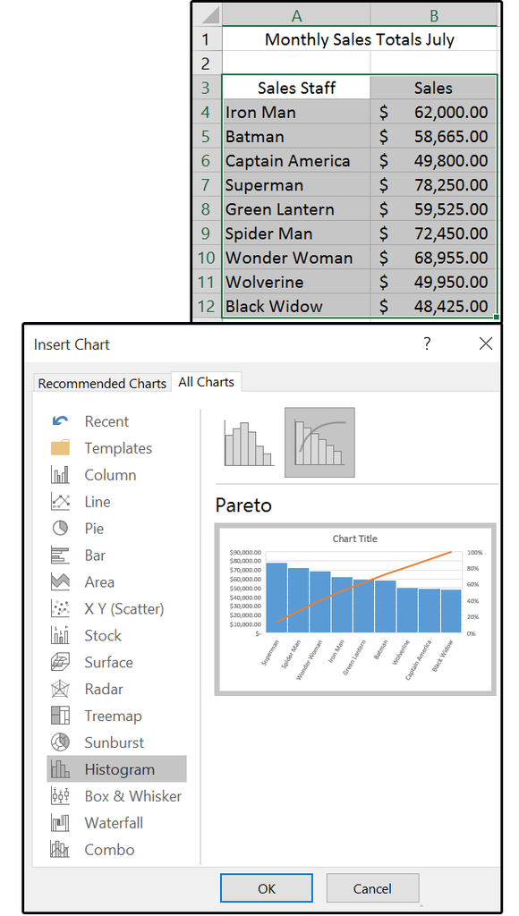
Pareto charts find the largest impact. They use both bars and a line graph. For example, individual values are represented in descending order by the bars, and the cumulative totals are represented by the lines. Use this chart to analyze data regarding the frequency of issues or causes in a process; to focus on the most significant of many issues or causes; or to analyze broad causes by studying their specific components.

1. Open your spreadsheet, highlight your table, then click Insert > Insert Statistical Chart > Pareto. The chart appears and opens the Chart Tools/Design Ribbon menus. Scroll across the Design options and select one that fits your project.

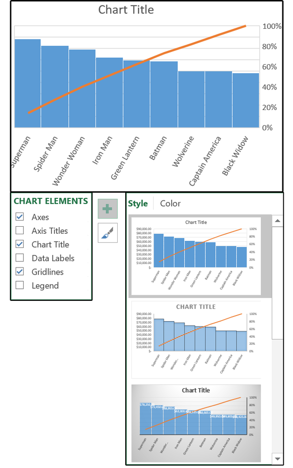
2. Click the + sign to edit the chart elements: Axes, Axes Titles, Chart Title, Data Labels, Gridlines, and Legend. Then click the paintbrush to change the chart’s style, design, and colors. The style changes are subtle, such as location of the legend or font attributes. Browse through the options and choose your favorite.

3. Right-click any of the rectangles on the chart and select Format Data Series. In the Format Data Series pane, click Series Options (the chart icon). Move the slider to change the gap width—that is, the space between each column on the chart.

4. Click the down arrow beside Series Options and browse through the drop-down menu to ascertain how each of these options perform. Select Horizontal Category Axis from the list.

5. Under Axis Options > Bins, select By Category. For Tick Marks, choose whether you’d like to see them inside or outside the chart, or Cross (both inside and outside), or other options. Then select Number and choose the number format you prefer from the list.

6. Next, select Chart Title from the Series Options dropdown menu, enter a new title, then adjust the alignment based on your preferences.

Again, notice how the chart has changed. Browse through the remaining options on the Series Options drop-down menu, including chart and plot areas, and axis settings. When finished, close the Format Data Series pane.

Waterfall shows value trends

Use Waterfall to show how initial values are affected by a sequence of positive and/or negative numbers. Waterfalls are also called Bridge, Flying Bricks, and Mario charts, because the intermediate-value columns appear to be floating in midair. A classic waterfall chart illustrates how an initial value is increased and decreased by a series of intermediate values, leading to a final value.

1. Access your spreadsheet and select the applicable database. Click Insert > Waterfall. The chart appears with the Chart Tools/Design Ribbon menus. Scroll across the Design options and select one with lots of obvious movement. Then click Colors and select a palette that has bright, contrasting colors (to illustrate the increased, decreased, and intermediate values most effectively).

2. Click the + sign to edit the chart elements: Axes, Axes Titles, Chart Title, Data Labels, Gridlines, and Legend. Then click the paintbrush to change the chart’s style, design, and colors. The style changes are subtle and include location of the legend and font attributes. Browse through the options and choose your favorite.

3. Right-click any of the rectangles on the chart and select Format Data Series. Browse through the options in this pane and make adjustments. (See the other charts for details regarding the Data Series options).

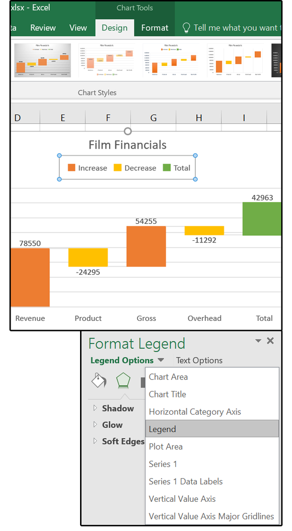
4. Right-click the chart again and select Format Legend > Legend, then enter the text labels that define the legend for this chart.

5. Double-click the last data point (the total or subtotal column) to open the Format Data Point pane. Check the Set As Total checkbox to make the column stationary, that is, not floating.

And that’s all for the new Histogram, Pareto, and Waterfall charts. Remember, we also covered the Treemap, Sunburst, and Box & Whisker charts.