Excel formula tips: How to troubleshoot by tracing dependents and precedents

When your spreadsheet has formulas piled on top of formulas, tracking and repairing errors would be agony if it weren’t for Excel’s Precedents and Dependents: cells that are referred to by a formula in another cell, and cells that contain formulas that refer to other cells, respectively. The next time you need to find out how the formula in C100 affects the formula in E175, which impacts the results in cell G225, try this technique. 

To view all the relationships between the cells in your spreadsheets, position your cursor on a cell with a formula that affects other cells (a Precedent) or choose a cell that contains information based on the results of other cells (a Dependent).

In this article’s example, open a spreadsheet with multiple formulas. Position your cursor on one of the formulas and press Ctrl+Shift+] (specifically: press and hold the Ctrl key and the Shift key with your left hand, then press the right bracket key with your right hand, then release all three keys).

In the following example, I placed the cursor on cell D15 (highlighted in yellow), then pressed Ctrl+Shift+]. Excel highlighted the cells D21 (YTD) and D22 (Average).

JD Sartain

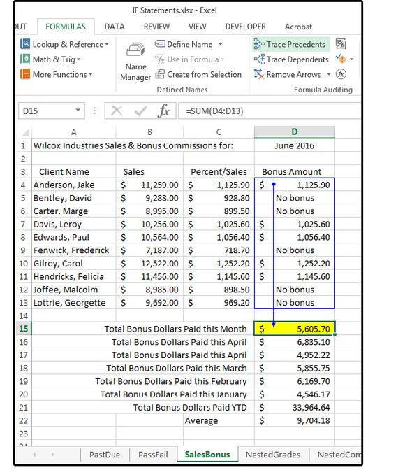
Move your cursor back to cell D15. Select Formulas > Formula Auditing and click the Trace Precedents button. In the screenshot below, notice the blue arrow (which shows the cells with no errors) begins at the top of column D (D4) and ends pointing to D15 (the initial cell that was selected). Red arrows indicate any cells that cause errors. Black arrows point to a spreadsheet icon indicating relationships in another spreadsheet, but only if that other spreadsheet is open.

JD Sartain

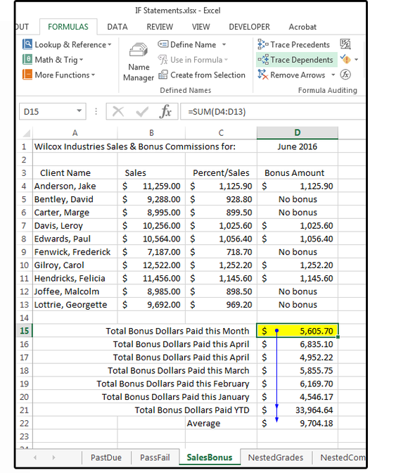
To identify the dependent cells, move the cursor back to cell D15, then select Formulas > Formula Auditing and click the Trace Dependents button. In the screenshot below, notice the blue arrow again. This time, it begins with the selected cell D15 and ends pointing to D21 and D22, because these two cells are “dependent” on the data in D15. In other words, without D15, there would be no data in D21 and D22.

To see the next (and remaining) levels that depend on the selected-active cell, click the Trace Dependents button twice.

JD Sartain

And last, for a quick view of all the relationships in a single spreadsheet:

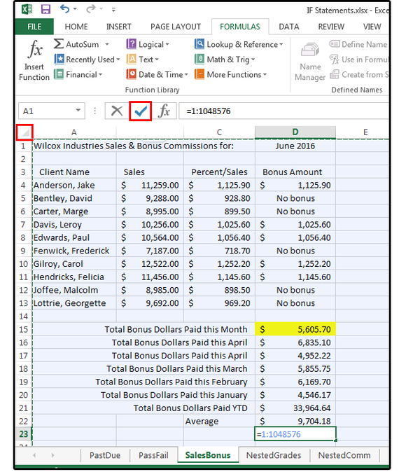
1. Move your cursor to an empty cell and enter the = (equal character).

2. Click the Select All button (the gray, arrow-like triangle in the top left corner of your spreadsheet, above the row numbers and beside the column letters and outlined in red in the screenshot below).

3. Click the checkmark in the formula bar (also outlined in red in the screenshot below). Ignore the warning about circular references—just click OK.

JD Sartain

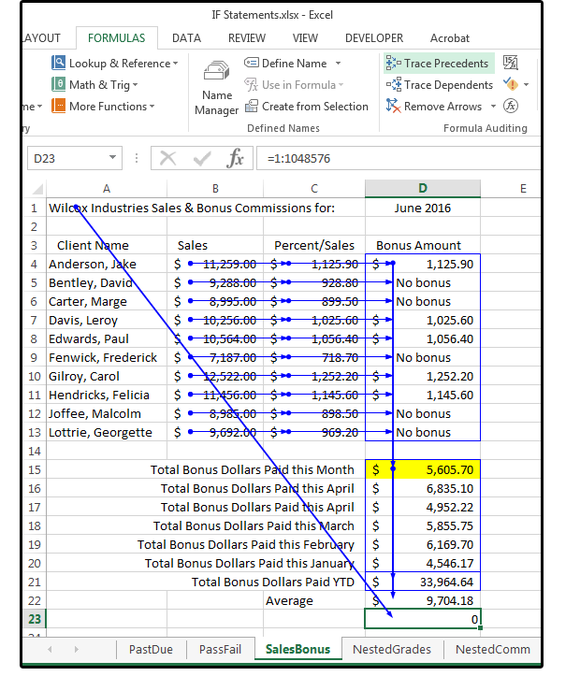
4. Once again, select Formulas > Formula Auditing. Click the Trace Precedents button twice, and all relationships are revealed.

5. When finished, delete the formula that appears in the formerly empty cell (= 1:1048576).

JD Sartain

We end with a housekeeping note: To remove arrows, select Formulas > Formula Auditing and click the Remove Arrows button.